What will you learn through this module?
- Valuations are crucial for businesses as they grow and evolve.
- Valuations help chart the course for the future by identifying the need for investments, expense reductions, or changes in the business.
- They also measure progress against strategic plans and identify gaps in non-financial aspects that drive value.
- Valuations have multiple purposes that extend beyond assessing the price of your business.
Introduction
The process of business valuation entails determining the monetary worth of a company or an asset. This involves gathering and evaluating various factors, including revenue, profits, and losses, as well as the risks and opportunities associated with the business. The objective is to determine an estimated intrinsic value for the company, allowing entrepreneurs and investors to make well-informed decisions regarding purchasing, selling, or investing.
Valuations are crucial for businesses as they grow and evolve. They provide a baseline, serving as a health metric for your business, indicating areas of improvement and measuring performance. Valuations help chart the course for the future by identifying the need for investments, expense reductions, or changes in the business. They also measure progress against strategic plans and identify gaps in non-financial aspects that drive value. Valuations empower effective business management, create accountability, and offer benchmarks for industry comparisons. Furthermore, they provide a perspective on price during transitions and serve as a gateway to securing capital. Lastly, valuations play a significant role in estate planning, allowing owners to better plan for their family's future. Overall, valuations offer valuable insights to strengthen and enhance the performance and value of a business.
Valuations have multiple purposes that extend beyond assessing the price of your business. They offer valuable insights into your business's internal operations, giving you a competitive advantage in enhancing its value and overall performance. In this module, we will explore various techniques for assessing value, including the residual income approach, multiples approach, dividend discount model, discounted cash flow approach, and economic value added.
Learning Objectives
The learning objective of business valuation involves developing a comprehensive understanding of the methodologies, principles, and techniques used to determine the intrinsic value of a business. It encompasses assessing and interpreting financial information, analyzing market conditions, and making informed judgments about a company's worth. This objective is crucial for investors, entrepreneurs, financial analysts, and professionals involved in mergers and acquisitions, as it enables them to make informed decisions regarding investments, transactions, and strategic planning.
To achieve the learning objective of business valuation, individuals should focus on the following:
- Grasp fundamental financial concepts: Understand the basics of financial statements, including balance sheets, income statements, and cash flow statements. This knowledge allows for evaluating a company's financial performance and identifying key indicators of value.
- Learn valuation methodologies: Acquire knowledge in different valuation techniques, such as discounted cash flow (DCF) analysis, which determines the present value of future cash flows, and comparable company analysis (CCA), which compares the target company with industry peers.
- Master valuation multiples: Gain proficiency in using the price-to-earnings (P/E) ratio and enterprise value-to-EBITDA (EV/EBITDA) ratio. These multiples offer a relative valuation perspective by comparing a company's financial metrics to industry benchmarks.
- Understand qualitative factors: Explore qualitative aspects that impact valuation, such as competitive advantage, market dynamics, and industry trends. Consider both quantitative and qualitative analyses to form a comprehensive understanding of a company's value.
In conclusion, the learning objective of business valuation involves acquiring a comprehensive understanding of financial analysis, valuation methodologies, and qualitative factors that impact a company's value. This knowledge empowers individuals to make informed investment decisions, assess potential acquisitions, and confidently engage in strategic planning.
Historical Approach
The historical approach in business valuation involves analysing past financial performance and historical data to determine the value of a business. This approach relies on historical financial statements, such as balance sheets, income statements, and cash flow statements, to assess the company's historical earnings, assets, liabilities, and cash flows.
Key elements of the historical approach in business valuation include:
- Financial Statement Analysis: The historical approach begins with thoroughly analyzing the company's financial statements. This involves examining revenue trends, profitability ratios, liquidity ratios, debt levels, and other relevant financial metrics to understand the company's past performance.
- Adjustments: In some instances, adjustments may be made to the historical financial statements to account for extraordinary items, non-recurring expenses, or one-time events that may distort the accurate picture of the company's economic performance.
- Comparative Analysis: Comparing the company's historical financial performance to industry benchmarks and similar companies can provide additional insights. This comparative analysis helps evaluate the company's historical performance relative to its peers and assess its competitive position.
- Historic Growth Rates: Calculating historical growth rates in revenue, earnings, and other financial indicators can help estimate the company's historical growth trajectory. This information can be used as a basis for forecasting future performance and projecting future cash flows.
- Market Conditions and Industry Analysis: Considering the company's historical performance within the context of market conditions and industry trends is essential. Evaluating the company's performance relative to market dynamics can provide valuable insights into its historical competitive position and growth potential.
While the historical approach helps understand a company's past performance, it may have limitations in predicting future performance. External factors and changes in the business environment may need to be adequately captured by historical data alone. Therefore, it is often combined with other valuation approaches, such as the income or market approach, to provide a more comprehensive and forward-looking assessment of a company's value.
Residual Income Approach
Residual income refers to the earnings generated by a company after considering its cost of capital, encompassing the combined expense of both debt and equity. Consequently, the residual income model aims to modify a company's projected future earnings to contain the equity cost, dividend payments, and other relevant equity expenses. Employing this approach allows analysts to derive a more precise valuation for a company.
The residual income model is a useful valuation tool for investors in specific scenarios. It is particularly applicable when valuing companies that do not pay dividends or generate positive cash flow. Unlike the DDM, it substitutes future residual income for dividends. Additionally, it differs from the DCF model by using the cost of equity instead of the weighted average cost of capital as the discount rate.
When should investors use the residual income model?
The residual income model is most effectively utilized when assessing the value of companies that do not distribute dividends or exhibit positive free cash flow.
The DDM (Dividend Discount Model) is a superior valuation method for dividend stocks. At the same time, the DCF (Discounted Cash Flow) approach is ideal for stocks that do not provide dividends but generate free cash flow. However, these valuation methods need to be revised for companies that fail to generate free cash flow, indicating their potential inability to afford dividend payments, as they lack the necessary inputs for those models. This is precisely where the residual income model excels, as investors can readily access the requisite data from a company's financial statements.
The pros and cons of the residual income model
The residual income model offers several advantages:
- It utilizes readily accessible data from a company's financial statements.
- It is a practical valuation approach for companies that do not distribute dividends or generate free cash flow.
- It emphasizes a company's economic profitability rather than solely focusing on its accounting profitability.
However, there are several limitations associated with this method:
- Valuation models better suited for companies that pay dividends or generate free cash flow are available.
- It heavily relies on forward-looking estimates, introducing a level of uncertainty.
- The cost of equity, a crucial input in the model, can be subjectively determined by an investor, potentially influencing the outcomes in a biased manner.
Multiples Approach
Investing necessitates substantial financial knowledge and a grasp of various valuation methodologies. One such approach is the multiples approach, founded on the straightforward notion that companies with similar assets tend to sell at comparable prices. It recognizes that financial metrics like cash flows and operating margins are universally applicable.
Understanding how these ratios operate is vital to ensure the viability of a potential investment. Moreover, it is an excellent means to compare different companies and identify those with the potential for higher returns on investment (ROI).
When employing the multiples approach, multiple indicators are considered to evaluate a stock. In essence, this approach entails analysing and comparing the financial metrics of companies within the same industry. By leveraging this method, analysts can determine the value of one business based on the value of another, delving into their operational and financial characteristics. This data and information can be utilized to make informed projections regarding expected growth.
What Are the Common Ratios Used in the Multiples Approach?
Valuation multiples can generally be classified into equity multiples and enterprise value multiples.
Equity multiples are particularly valuable for investors with minority company positions, as they primarily focus on evaluating the equity value. Here are some commonly used equity multiples:
- P/E ratio (Price-to-Earnings ratio): This is a widely utilized equity multiple due to the extensive data availability. It calculates the ratio between a company's share price and earnings per share (EPS).
- Price-to-sales ratio: This ratio is straightforward and can be applied to companies incurring losses. It compares the share price to the sales revenue per share.
- Price-to-book ratio: This ratio can benefit industries where assets significantly contribute to earnings. It is calculated by dividing the share price by the book value per share.
- Dividend yield: This ratio enables the comparison of cash returns across different investment types. It is determined by dividing the dividend per share by the share price.
Enterprise value multiples are particularly valuable in scenarios such as mergers and acquisitions, as they help mitigate the impact of debt financing. Here are some commonly used enterprise value multiples:
- Revenue ratio: This ratio may be influenced by variations in accounting practices. It is calculated by dividing the enterprise value by sales or revenue, providing insight into the proportion of enterprise value relative to the company's sales.
- EBITDA ratio (Earnings Before Interest, Tax, Depreciation, and Amortization): This ratio is frequently utilized in the hotel and transportation industries. It compares the EBITDA with the enterprise value, shedding light on the relationship between operating earnings and enterprise value.
Even in cases where there is no alteration in the enterprise value, equity multiples can be utilized to assess the impact of changes in the capital structure.
Dividend Discount Model
When you purchase publicly traded stock, the only form of cash flow you receive from the company is in the form of dividends. The dividend discount model (DDM) is an uncomplicated valuation approach that assesses the worth of stock by computing the present value of anticipated dividends. Investors typically expect two types of cash flows when they buy stocks: dividends received during the holding period and an anticipated price at the end of that period.
By summing up all future dividend payments and discounting them to their present value, the dividend discount model (DDM) utilizes a quantitative methodology to predict the stock price of a company. It aims to estimate the fair value of stock regardless of market conditions, considering factors such as dividend pay-out and expected market returns. If the value derived from the DDM exceeds the current trading price of shares, it suggests that the stock is undervalued and may be a good buy, and vice versa.

The dividend discount model can be implemented in various forms, each relying on specific assumptions. Here are some notable variations:
- The Gordon Growth Model, referred to as GGM, is a popular variant of the dividend discount model widely utilized in practice. It enables investors to assess the intrinsic value of a stock by considering the expected constant growth rate of dividends.
According to the GGM, it is presumed that dividend payments will experience an everlasting, constant growth rate in the future. It is particularly useful for valuing stable businesses with consistent cash flow and predictable dividend growth. In this model, it is assumed that the company under evaluation maintains a consistent business model and experiences growth at a steady and unchanging rate throughout time. Mathematically, the GGM is represented as follows:
Gordon Growth Model -

Value at time 0 = Dividend at time 1 / Cost of equity - Constant growth rate
Where:
V0 - Current value of the stock
D1 - Dividend payment expected in next period
R - Estimated cost of equity capital calculated using the Capital Asset Pricing Model (CAPM)
g - Constant growth rate
Example: There is a company whose stock is trading at $110 per share. This company has a minimum required rate of return (r) of 8%, and it is expected to pay a $3 dividend per share next year (D1), with an annual growth rate (g) of 5%.
To calculate the intrinsic value (V) of the stock, we can use the Gordon growth model formula:
V = D1 / (r - g)
Substituting the given values, we get:
V = $3 / (0.08 - 0.05)
V = $3 / 0.03
V = $100
According to the Gordon growth model, the intrinsic value of the stock is $100 per share. Since the current market price is $110, the shares are considered to be overvalued by $10.
- One period DDM model
The frequency of using the one-period discount dividend model is lower when compared to the Gordon Growth model. It is typically employed when an investor wishes to calculate the intrinsic value of a stock that they intend to sell within a single period, usually one year.
The one-period DDM assumes that the investor plans to hold the stock for only a year. Due to this short holding period, the expected cash flows from the stock consist of a single dividend payment and the selling price of the stock.
Hence, to ascertain the suitable price for the stock, it is necessary to calculate the present value of the combined future dividend payment and estimated selling price after discounting them.

Where:
- V0 – The current fair value of a stock
- D1 – The dividend payment in one period from now
- P1 – The stock price in one period from now
- r – The estimated cost of equity capital
Example: ABC Corp. will distribute $3 as dividends per share, and the projected selling price at the end of the holding period is anticipated to be $120 per share.


The estimated cost of equity capital is 5%. At present, the stock of ABC Corp. is trading at $118 per share.
The intrinsic value of the stock is calculated to be $117.14, which is lower than the current stock price of $118. Consequently, we can conclude that the stock is presently overvalued.
- Multi-Period Dividend Discount Model
The multi-period dividend discount model is an expansion of the one-period dividend discount model, specifically utilized when investors have intentions to hold a stock over multiple periods. The main hurdle in the multi-period model lies in accurately predicting dividend payments for each individual period.
In the multi-period DDM, the investor anticipates holding the purchased stock for multiple time periods.
In this method expected future cash flows include multiple dividends and the projected selling price at the end of the holding period. To find the intrinsic value of a stock using this model, one needs to estimate the combined value of these dividends and selling price, discounted to their present values.

Example: ABC Inc. expects dividends of $2 and $2.5 at the end of the next two years, respectively. The expected stock price at the end of year 2 is $48. If the required rate of return is 15%, then the value of ABC’s share today is closest to:

Discounted Cash Flow Approach
Discounted Cash Flow is a valuation technique that helps to determine whether an investment is worthwhile based on projected future cash flows. It estimates the value of an investment using its projected future cash flows.
The main principle of finance is that $1 today is worth more than $1 a year from now. This principle is called the "time value of money" concept and is a significant base for DCF valuation. Projected future cash flows need to be discounted to present value, so they can be correctly analysed.
This valuation technique is used to determine if an investment is worth it in the long run. For example, in investment banking, a DCF is used to decide whether a prospective merger or acquisition is worth it. Moreover, DCF valuation is used in real estate and private equity.
What is Discounted Cash Flow Valuation formula?
The formula of DCF is:
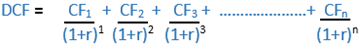
CFâ‚ = Cash flow for the first period
CFâ‚‚ = Cash flow for the second period
CFâ‚™ = Cash flow for “n” period
n = Number of periods
r = Discount rate
Cash Flow:
Cash flow means the money created by the company that is available to be reinvested in the business or distributed to investors. It can be a sort of earnings or dividend.
Number of periods:
The number of periods is the no. of years, in which the cash flows are anticipated to generate.
Discount Rate:
The discount rate brings future cash flow to present value. Usually, the discount rate is the company's cost of capital or how much the company should earn to bear the cost of operation. This is usually the weighted average cost of capital, which is the company's interest rate and loan payments or dividend payments to shareholders.
DCF Valuation Example:
Let's say you have a company and are planning to begin a big project. Your company’s weighted average cost of capital is 7%, so you’ll use 7% for your discount rate. The project is set to last for five years, and your company needs to put in an initial investment of $15 million. Future cash flows for the project are:
- Year 1: $1 million
- Year 2: $3 million
- Year 3: $5 million
- Year 4: $5 million
- Year 5: $7 million
So, if you will put these future cash flows and your 7% discount rate in the formula, your yearly discounted cash flows are:

Note: Discounted cash flow numbers are rounded to the nearest whole dollar amount.
Now to check whether the project is valuable or not, you need to compare the initial investment (Project investment) with the total Discounted Cash Flows over the project's life. So here:
- Initial Investment: $15,000,000
- Total Discounted Cash Flows: $16,441,764
- Net Present Value of the project: $16,441,764 - $15,000,000 = $14,41,764
Net present value is the difference between the project's initial investment and the discounted cash flows sum. If this amount is positive, it is worth investing in a project; otherwise, it is not.
Here the $1,441,764 is a positive number, implying that the money generated by the project is more than the initial investment. So, your company can invest in this project.
Economic Value Added
EVA, which stands for Economic Value Added, is a performance measure that evaluates the generation of shareholder value. It sets itself apart from conventional financial performance metrics like net profit and earnings per share (EPS).
EVA computes the residual profits that are left over after subtracting the capital costs, encompassing both debt and equity, from a company's operating profit. The underlying concept is straightforward yet robust: genuine profitability should consider the cost of capital.
Example: Company X has a capital of $200 million, encompassing both debt and shareholder equity. The cost of utilizing that capital, including interest on debt and the cost of underwriting the equity, amounts to $15 million annually. For Company X to create economic value for its shareholders, profits must exceed $15 million per year. If Company X earns $25 million, the resulting EVA would be $10 million
EVA Calculation
There are four steps in the calculation of EVA:
- Calculate Net Operating Profit After Tax (NOPAT)
- Calculate Total Invested Capital (TC)
- Determine the Weighted Average Cost of Capital (WACC)
- Calculate EVA
EVA = NOPAT – WACC * TC

To put it differently, EVA incorporates a "rent" concept where the company is charged for utilizing investors' funds to sustain its operations. This "rent" compensates investors for forgoing the opportunity to use their own money elsewhere. EVA effectively captures this concealed cost of capital that is often overlooked by conventional measures
EVA can be calculated using the formula: EVA = NOPAT - (WACC × Capital)
First, we need to calculate the components of EVA.
NOPAT (Net Operating Profit After Tax) is calculated by multiplying the operating income by (1 - Tax Rate).
Example: NOPAT for Company XYZ is $500,000 for the current financial year.
The calculated WACC (Weighted Average Cost of Capital) for Company XYZ is 10% for the same year.
The total capital invested, which includes both debt and equity, amounts to $4 million for Company XYZ.
Now, we can plug these values into the EVA formula to calculate the EVA.
EVA = NOPAT - (WACC × Capital) EVA = $500,000 - (10% × $4,000,000)
EVA = $500,000 - $400,000
EVA = $100,000
Based on the calculation, the economic value added (EVA) by Company XYZ is $100,000. This positive value indicates that Company XYZ is effectively utilizing its invested capital and generating sufficient economic value.